 Optimization ToolOptimization Tool
The Optimization tool solves linear programming (LP), mixed integer linear programming (MILP), and quadratic programming (QP) optimization problems using matrix, manual, and file input modes.
This tool uses the R programming language. Go to Options > Download Predictive Tools to install R and the packages used by the R Tool.
Optimization has wide applications in many industries, such as supply chain, transportation, financial services, retail, telecommunications, and energy. Application areas include supply chain optimization, assortment optimization, portfolio optimization, workforce scheduling, and sports scheduling.
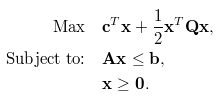
An optimization problem typically has the following mathematical form, consisting of an objective function (first equation), a set of constraints (second equation), and a specification of the types (continuous, integer, binary) and bounds of the decision variables (third equation). The goal is usually to find the values of the decision variables that maximize or minimize the objective, while satisfying all the underlying constraints, types and bounds.
No inputs are required for the manual or file input modes. For the matrix input mode, inputs O and A are required (B and Q are optional).
variable: (Required) a string, decision variable names. Corresponds to x in the equations.
coefficient: (Required) a number, coefficient of each decision variable in objective function. Corresponds to c.
lb: (Optional) a number, lower bound of the decision variable. The default value is 0.
ub: (Optional) a number, upper bound of the decision variable. The default value is Inf (positive infinity).
type: (Optional) a character, the type of the decision variable, which can be C (continuous), B (binary), or I (integer). The default value is C.
Beginning with Alteryx 11.0, you can enable the Display field mapping for Input Anchor O option for more flexibility with field names.
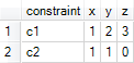
Constraints in rows: Each row corresponds to a constraint. The first field can optionally be named constraint to indicate the constraint name in each row, while the remaining field names should correspond to the decision variables defined in O. Additionally, you can include the fields dir and rhs to roll the B input into this.
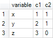
Variables in rows: Each row corresponds to a variable. The first field should be named variable, while the remaining field names should correspond to the constraint names. Note that this corresponds to the transpose of the A matrix in the above equations.
The order of variables for input O and input A should be the same.
Beginning with Alteryx 11.0, you can use other field names for âconstraintâ or âvariableâ and the Optimization tool will intelligently infer which field contains constraints and which field contains variables. However, Alteryx recommends that you follow the naming convention.
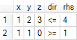
B: (Required if not already provided in A) Use this input to provide the name, direction, and right hand side of the constraints.
constraint: (Optional) a string, name of the constraint.
dir: a string, direction of the constraint inequality. It has to be >=, <= or ==.
rhs: a number, the right hand side of the inequality, corresponding to b.
Q: (Optional) Use this input to provide the quadratic portion of the objective function, for Quadratic Programming problems. It corresponds to Q in the equations. You can specify it as a dense matrix or as a sparse matrix.
Dense matrix: The field names should correspond to the decision variable names defined in O.
Sparse matrix: The field names are i, j, and v, where i and j are row and column indexes, respectively, and v is the non-zero value of the associated matrix element.
©2018 Alteryx, Inc., all rights reserved. Allocate®, Alteryx®, Guzzler®, and Solocast® are registered trademarks of Alteryx,